A1. Displaying multiple scalar summaries on the same plot in TensorFlow/TensorBoard
I assume that my readers have some basic knowledge about TensorFlow - primarily how to set up summary ops in the computation graph to prepare a TensorBoard session. If you are unfamiliar with TensorBoard, there exists some excellent documentation here which you should check out before continuing with this tutorial.
When training neural networks, we usually split our available data into three separate files: training, validation, and test data. In order to gauge the stability of the network architecture, it is good to visualize how your network performs against the validation data after every x iterations of training. TensorBoard provides us with some great visualization tools to observe how values like the training cost and cross-validation cost evolve through the training process. The code snippet below shows the traditional way to set up a scalar summary to track the training cost through the training.
# some other ops and variables set up previously ...

cost = tf.losses.mean_squared_error(labels, logits)

tf.add_to_collection('cost', cost)

tf.summary.scalar('cost', cost)

train_op = optimizer.minimize(cost)

# maybe you've set up some other summaries previously...
# merge them all into one single op!

summary_op = tf.summary.merge_all()
You typically set up a FileWriter object (which I will constantly refer to as a ‘summary writer’) in your TensorFlow session to save the summaries to disk, and reference them from the command line when opening TensorBoard.
with tf.Session(graph=my_graph) as sess:
  writer = tf.summary.FileWriter(your_summary_directory, sess.graph)
  # stuff
  # ...
  # ...
  summary, _ = sess.run([summary_op, train_op])
  writer.add_summary(summary)
  # more stuff
  # ...
  # ...
Now when you open up TensorBoard, you can see your cost function plotted in the Scalars section.
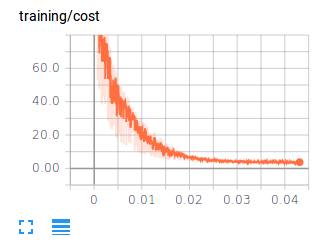
We see that our cost function is decreasing, which is good! But, is the network really learning, or is it just curve-fitting the training data? Let’s set up a summary for our validation error. The following snippets will be a bit more detailed this time around.
global_step = tf.Variable(0, trainable=False, dtype='int64')
tf.add_to_collection('global_step', global_step)

cost = tf.losses.mean_squared_error(labels, logits)
v_cost = tf.losses.mean_squared_error(v_labels, v_logits)

tf.add_to_collection('cost', cost)
tf.add_to_collection('v_cost', v_cost)

tf.summary.scalar('cost', cost,
                  collections=['training_summaries'])

tf.summary.scalar('validation_cost', v_cost,
                  collections=['validation_summaries'])

train_op = optimizer.minimize(cost)
tf.add_to_collection('train_op', train_op)

training_summary_op = tf.summary.merge_all('training_summaries')
validation_summary_op = tf.summary.merge_all('validation_summaries')

tf.add_to_collection('training_summary_op', training_summary_op)
tf.add_to_collection('validation_summary_op', validation_summary_op)
Here, instead of using the generic GraphKeys collection, we assign the training summary ops and validation summary ops their own proper collections. We also replace the generic merge_all call (which assumes the summary ops to merge are all in the defaults GraphKeys collection) with two separate ‘merge_all’ calls, each referring to the unique collections we created. This will ensure all the summary operations in the graph will be executed in the correct fashion.
Now from the module from which we are running our training, we run the training summary op after every training iteration, and the validation summary op after every x training iterations. Here I’ve chosen x = 3.
train_op = my_graph.get_collection('train_op')[0]
cost = my_graph.get_collection('cost')[0]
training_summary_op = my_graph.get_collection('training_summary_op')[0]
validation_summary_op = my_graph.get_collection('validation_summary_op')[0]
global_step = my_graph.get_collection('global_step')[0]

with tf.Session(graph=my_graph) as sess:
    writer = tf.summary.FileWriter(your_summary_directory, sess.graph)

    _global_step = sess.run(global_step)

    while _global_step < FLAGS.max_steps:
        if (_global_step + 1) % FLAGS.update_freq == 0:
            if (_global_step + 1) % 3 * FLAGS.update_freq == 0:
                _global_step, summary = sess.run([global_step,
                                             validation_summary_op])
                writer.add_summary(summary)
            else:
                _global_step, summary, _ = sess.run([
                                           global_step,
                                           training_summary_op,
                                           train_op])
                writer.add_summary(summary)
        else: _global_step, _ = sess.run([global_step, train_op])

    # do some other stuff before finishing up, then close...
    writer.close()
In TensorBoard, we now have two plots - one for training accuracy, and one for cross-validation accuracy (with 1/3 as many points).
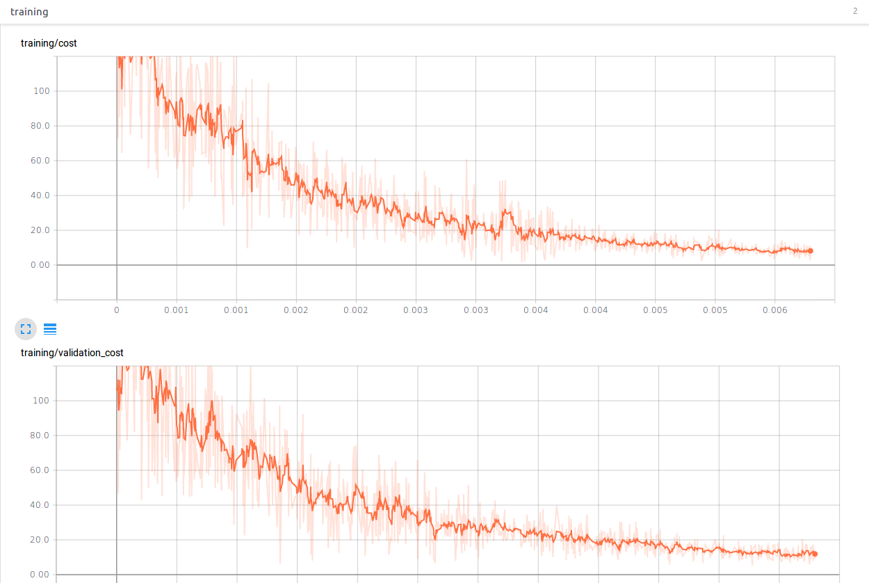
In this image the training data and validation data follow a very similar curve. But, how do we plot both the validation and training cost on the same plot? We would really love to do this in order to have a better visualization of the ‘turning point’, so-to-speak, or the point in the training at which our cross-validation accuracy begins to diverge from our training accuracy.
The short answer is: you can’t. TensorFlow does not currently support this type of feature, namely adding two scalar summaries to the same plot. However, after much tweaking and hacking, I’ve found a reliable, albeit slightly cumbersome, way to accomplish this.
We first need to add some additional ops and variables to our graph. They are as follows:
# ... previous graph code above ...#

dummy_cost = tf.Variable(0.0)
tf.add_to_collection('dummy_cost', dummy_cost)

dummy_summary_op = tf.summary.scalar('dummy_summary', dummy_cost)

tf.add_to_collection('dummy_summary_op', dummy_summary_op)
Next, in the module where we are running our training, we will need to set up two summary writers, instead of just one.
with tf.Session(graph=my_graph) as sess:
  train_writer = tf.summary.FileWriter(train_directory, sess.graph)
  validate_writer = tf.summary.FileWriter(validate_directory, sess.graph)
Now, when we write test data, we will use the train_writer, and when we write validation data, we will use the validation_writer. So the code we had before (with accessors to our new ops and variables) becomes,
train_op = my_graph.get_collection('train_op')[0]
cost = my_graph.get_collection('cost')[0]
v_cost = my_graph.get_collection('v_cost')[0]
training_summary_op = my_graph.get_collection('training_summary_op')[0]
validation_summary_op = my_graph.get_collection('validation_summary_op')[0]
global_step = my_graph.get_collection('global_step')[0]

dummy_cost = my_graph.get_collection('dummy_cost')[0]
dummy_summary_op = my_graph.get_collection('dummy_summary_op')[0]

with tf.Session(graph=my_graph) as sess:
    train_writer = tf.summary.FileWriter(train_directory, sess.graph)
    validate_writer = tf.summary.FileWriter(validate_directory, sess.graph)

    _global_step = sess.run(global_step)

    while _global_step < FLAGS.max_steps:
        if (_global_step + 1) % FLAGS.update_freq == 0:
            if (_global_step + 1) % 3 * FLAGS.update_freq == 0:
                _global_step, summary = sess.run([global_step,
                                             validation_summary_op])
                validate_writer.add_summary(summary)
            else:
                _global_step, summary, _ = sess.run([
                                           global_step,
                                           training_summary_op,
                                           train_op])
                train_writer.add_summary(summary)
        else: _global_step, _ = sess.run([global_step, train_op])
Before we get to why we created the dummy variable, let me first explain the implications of using two summary writers. When you go to launch TensorBoard now, the command is slightly different, because you want TensorBoard to read from two directories simultaneously. It’s pretty simple:
$ tensorboard --logdir=x:path/to/train_dir,y:path/to/validate_dir
Now, because the validation and training scalar summaries are coming from two different summary writers, the plots will contain curves of different color.
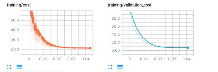
In order to get these curves on the same plot, we are going to use our dummy_cost variable and dummy_summary_op.
if (_global_step + 1) % 3 * FLAGS.update_freq == 0:
    _global_step, summary, _cost, _v_cost = sess.run([global_step,
                                             validation_summary_op,
                                             cost, v_cost])
    validate_writer.add_summary(summary)
    _ , dummy_summary = sess.run([dummy_cost,
                                           dummy_summary_op],
                                  feed_dict = {dummy_cost: _cost})
    train_writer.add_summary(dummy_summary)
    _ , dummy_summary = sess.run([dummy_cost,
                                           dummy_summary_op],
                                  feed_dict = {dummy_cost: _v_cost})
    validate_writer.add_summary(dummy_summary)
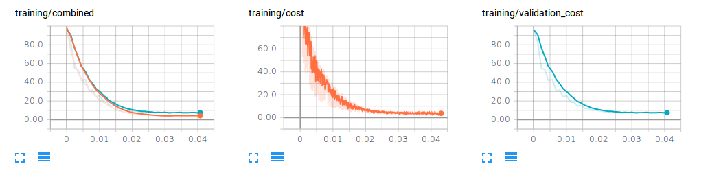
We simply capture the current training cost and current validation cost in two local variables, and sequentially feed those values to the dummy_cost variable via a feed dictionary, writing to each summary writer in between.
Because two different summary writers are writing a summary with the same name attribute, they will now appear on the same plot in your scalars section.
TL;DR : In your graph, construct a dummy cost variable separate from your validation and training cost variables and initialize it as zero-valued. In your session, create two file writers, each pointing to different directories. Where you normally run the validation cost, also run the training cost (without the training op), and retrieve the output of both validation cost and training cost. Use a feed dictionary to feed the cost output into the dummy cost variable, and write to the first summary writer. Repeat with the validation cost output, and write to the second summary writer. When you run TensorBoard now, point to both summary directories you used in your summary writers. Now you will have both training and cross-validation data on the same plot.
Hope this helps! Happy TensorFlowing.